Because of its specific needs, the rocket industry has developed its own pump design approaches which may differ from those for conventional applications. In addition, designers may employ their individual methods of analysis and calculation. However, the broad underlying principles are quite similar. The range of speeds, proportions, design coefficients, and other mechanical detail for rocket engine pumps has been well established by earlier designs as well as through experiments.
As a rule, rated pump head-capacity ( H−Q ) requirements and expected available NPSH at the pump inlets will be established by engine system design criteria. The first step then is to choose a suitable suction specific speed ( NSS ) and the type of inducer which will yield the highest pump speed ( N ) at design conditions (eq. (6-10)). The pump specific speed (NS) or type of impeller can now be established from the chosen pump speed and required head-capacity characteristics. Owing to its relatively light weight and simplicity of construction, a singlestage centrifugal pump may be given first consideration.
With suction specific speed and specific speed of the proposed pump design established, the designer can now look for a suitable "design model" among comparable existing pumps which approximate the desired performance. The latter includes satisfactory suction requirements, suitable head-capacity characteristics, and acceptable efficiency. If a suitable model is available, the design calculations of the new pump will include application of a scaling factor to the parameters of the existing model. The following correlations are valid for pumps with like specific speed, based on the pump affinity laws (eqs. (6-6a) and (6-6b)):
ΔH1= rotating speed (rpm), flow rate (gpm), and developed head (ft) of the existing model at rated conditions
N2,Q2, and
ΔH2= rotating speed (rpm), flow rate (gpm), and developed head ( ft ) of the new pump at rated conditions
f=D2/D1
= scaling factor
D1
=impeller diameter of the existing model, ft
D2
= impeller diameter of the new pump, ft
This approach assumes that other dimensions of the pump are in approximately linear proportion to the impeller diameter.
If a suitable model is not available for the design of a new pump, the designer can use "design factors" established experimentally by other successful designs. These may permit establishing relations between rated pump developed head and flow rate, and such parameters as velocity ratios. However, best results are obtained through experimental testing of proposed design itself. The test results then are used for design revisions and refinements.
In the discussions below, the following basic symbols are used:
c=flow velocities, absolute (relative to ducts
    and casing)
v=flow velocities, relative to inducer or im-
    peller
u=velocities of points on inducer or impeller
Subscript:
0 = inducer inlet
1 = inducer outlet = impeller inlet
2 = impeller outlet
3 = pump casing
prime 1 = actual or design
Operating Principles of the Centrifugal Pump Impeller
In its simplest form, the impeller of a centrifugal pump can be regarded as a paddle wheel with radial vanes, rotating in an enclosure, with the fluid being admitted axially and ejected at
the periphery. This is shown schematically in figure 6-33. The tangential velocity component of each fluid element increases as it moves out radially between the vanes. Therefore, the centrifugal force acting on these fluid elements increases as the fluid moves out radially. Assuming constant flow velocity in the radial direction and no energy losses, the ideal head rise due to centrifugal force between the central entrance (1) and the peripheral exit (2) is
ΔHic=2gω2(r22−r12)(6-25)
where
ΔHic=ωr1=r2=g ideal head rise due to centrifugal forces, ft= angular velocity of the wheel, rad/sec vane radius at the entrance, ft vane radius at the periphery, ft= gravitational constant, 32.2ft/sec2
For optimum performance, most impellers in high-speed centrifugal rocket engine pumps have shrouded, backward curved vanes. The impeller width is tapered toward the periphery to keep the cross-sectional area of the radial flow path near constant. A typical impeller design of this type is shown in figure 6-34.
Velocity diagrams may be constructed to analyze the fluid flow vector correlations at various points of an impeller. Let us assume the following ideal conditions:
(1) There are no losses, such as fluid-friction losses
(2) The impeller passages are completely filled with actively flowing fluid at all times
Figure 6-33.-Paddle wheel (schematic).
Figure 6-34.-Typical shrouded centrifugal impeller with backward curved vanes.
(3) The flow is two dimensional (velocities at similar points on the now lines are uniform)
(4) The fluid leaves the impeller passages tangentially to the vane surfaces (complete guidance of the fluid at the outlet)
The ideal inlet (point (1)) and outlet (point (2)) flow velocity diagrams of the impeller described in figure 6-34 are shown in figure 6-35. At this point with corresponding fluid velocities u,v, and c (as identified above), α is the angle between c and u, and β is the angle enclosed by a
INLET VELOCITY DIAGRAM
OUTLET VELOCITY DIAGRAMS
Figure 6-35.-Flow velocity diagrams for the impeller shown in figure 6-34 (draw in a plane normal to the impeller axis).
tangent to the impeller vane and a line in the direction of vane motion. The latter is equal to the angle between v and u (extended).
Based on these velocity diagrams, the following correlations have been established: 1
ΔHip= ideal static pressure head rise of the fluid flowing through the impeller due to centrifugal forces and to a decrease of flow velocity relative to the impel- ler, ftΔHi= ideal total pressure head rise of the fluid flowing through the impeller = the ideal developed head of the pump impeller, ftQimp= impeller flow rate at the design point (rated conditions), gpm A1= area normal to the radial flow at the impeller inlet, ft2cm1= "meridional" or (by definition for radial flow impellers) radial component of the absolute inlet flow velocity, ft/sec
For pumping low-density propellants (such as liquid hydrogen), which is associated with very high developed heads, straight radial vanes are frequently used in centrifugal impellers, since they permit a higher obtainable head coefficient ψ. Figure 6-36 presents a typical radial vane impeller and its outlet velocity diagram. The vane discharge β2=90∘ and cy2=u2. The ideal developed head of a radial vane impeller becomes
ΔHi=gu22−u1cu1(6-29)
For centrifugal pumps of the noninducer type (which are now rarely used in rocketry), proper selection of the impelier inlet vane angle β1 or the provision of guide vanes at the inlet minimizes the absolute tangential component of fluid flow at the inlet, cu1, which for best efficiency should be zero. This is defined as no prerotation, where a1=90∘. Thus, equation (6-26) becomes
ΔHi=gu2cu2(6-30)
Figure 6-36.-Typical radial vane impeller and its outlet velocity diagram.
The above discussions assumed ideal conditions. For most rocket applications, centrifugal pumps are designed with an inducer upstream of and in series with the impeller. The flow conditions at the impeller inlet thus are affected by the inducer discharge flow pattern. In addition, two types of flow usually take place simultaneously in the flow channels; namely, the main flow through the passages, and local circulatory flows (eddy currents). The latter are relatively small but modify the former. The resultant effect at the impeller inlet is to make the flow enter at an angle β1′, larger than the impeller inlet vane angle β1. The fluid is also caused to leave the impeller at an angle β2′, less than the impeller discharge vane angle β2, and to increase the absolute angle α2 to α2′. This and the hydraulic losses in the impeller correspondingly change the relative flow velocities v1 and v2 to v1′ and v2′, the absolute flow velocities c1 and c2 to c1′ and c2′, and the absolute tangential components cu1 and cu2 to cu1′ and cu2′. Since the radial flow areas A1 and A2, and the impeller flow rate Qimp remain constant, the absolute radial or meridional components cm1 and cm2 also remain unchanged. The inlet and outlet flow velocity diagrams in figure 6-35 may now be redrawn as represented by the dotted lines.
The correlation established in equation (6-26b) may be rewritten as
ΔHimp=gu2cu2′−u1cu1′(6-31)
where
ΔHimp=cu1′=cu2′= impeller actual developed head, ft tangential component of the design absolute inlet flow velocity, ft/sec tangential component of the design absolute outlet flow velocity, ft/sec
The ratio of the design now velocity cu2to the ideal flow velocity cu2 can be expressed as
ev=cu2cu2′(6-32)
where ev= impeller vane coefficient. Typical design values range from 0.65 to 0.75.
Referring to figure 6-35, equation (6-28) may be rewritten as
cu2′=u2−tanβ2′cm2(6-33)
By definition, the required impeller developed head can be determined as
ΔHimp=ΔH+He−ΔHind(6-34)
where
ΔH=ΔHind =He= rated design pump developed head, ft required inducer head-rise at the rated design point, ft hydraulic head losses in the volute, ft. Typical design values of He vary from 0.10 to 0.30ΔH.
The required impeller flow rate can be estimated as
Qimp=Q+Qe(6-35)
where
Qimp =QQe= required impeller flow rate at the rated design point, gpm rated delivered pump flow rate, gpm impeller leakage losses, gpm. Most of these occur at the clearance between impeller wearing rings and casing. Typical design values of Qe vary from 1 to 5 percent of Qimp .
After general pump design parameters, such as developed head ΔH, capacity Q, suction specific speed NSS , rotating speed N, and specific speed NS have been set forth or chosen, the design of a centrifugal (radial) pump impeller may be accomplished in two basic steps. The first is the selection of those velocities and vane angles which are needed to obtain the desired characteristics with optimum efficiency. Usually this can be achieved with the help of available design or experimental data such as pump head coefficient ψ, impeller vane coefficient ev, and leakage loss rate Qe. The second step is the design layout of the impeller for the selected angles and areas. Considerable experience and skill are required from the designer to work out graphically the best-performing configuration based on the given design inputs.
The following are considered minimum basic design elements required for proper layout of a radial-flow impeller:
1.Radial velocity at the impeller entrance or eye,cm1 .-This is a function of inlet conditions such as inducer discharge velocity and inlet duct size.For best performance,the value of cm1 should be kept reasonably low.Typical design values of cm1 range from 10 to 60ft/sec .
2.Radial velocity at the impeller discharge, cm2 .-Its value is a function of the impeller peripheral velocity u2 and the flow coefficient ϕ . Typical design values for cm2 range from 0.01 to 0.15u2 .
3.Diameter of the impeller at the vane en- trance,d1 .-Its value is determined by the in- ducer design as well as by impeller shaft and hub size.
4.The impeller peripheral velocity at the discharge,u2 .-The value of u2 can be calcu- lated by equation(6-4)for a given pump devel- oped head H and a selected overall pump head coefficient,ψ .The maximum design value of u2 is often limited by the material strength which thus determines the maximum developed head that can be obtained from a single-stage impel- ler.Typical design values of u2 range from 200 to 1500ft/sec .With u2 and N known,the impel- ler discharge diameter d2(in)can be calculated readily.
5.The inlet vane angle β1 .The value of β1 is affected by the inlet flow conditions.Gener- ally,β1 should be made equal or close to the inlet flow angle β1′ which can be approximated by
tanβ1′=cm1/(u1−cu1′)(6-36)
Typical design values for β1 range from 8∘ to 30∘ .
6.The discharge vane angle β2 .-In the special case of radial vane impeller designs β2=90∘ .For backward curved vane impellers, β2 is the most important single design element. Usually the selection of β2 is the first step in determining the other impeller design constants, since most of them depend on β2 .Pump effi- ciency and head-capacity characteristics are important considerations for the selection.For a given u2 ,head and capacity increase with β2 . Typical design values for β2 range from 17 to
28∘ ,with an average value of 22.5∘ for most specific speeds.
Figure 6-37 presents the basic layout of a typical radial-flow impeller with backward curved vanes.The shaft diameter ds may be determined by the following correlations
where
ds= impeller shaft diameter,in
T= shaft torque corresponding to yield or ultimate loads as defined by equations (2-9)and(2-10),lb-in
M= shaft bending moment corresponding to yield or ultimate loads as defined by equations(2-9)and(2-10),1b-in
Ss= shear stress due to torque, lb/in2St= tensile stress due to bending moment, lb/in2SSW= allowable working shear stress(yield or ultimate)of the shaft material, lb/in2Stw= allowable working tensile stress(yield or ultimate)of the shaft material, lb/in2
Impeller hub diameter dh and eye diameter de may be equal to hub diameter and tip diameter of the inducer.The maximum tensile stress in- duced in an impeller by the centrifugal forces
Figure 6-37.-Basic layout of a typical radial- flow impeller with backward curved vanes.
occurs as the tangential stress at the edge of the shaft hole. It may be checked by
St max =gKs=ρμds=d2=u2 max = maximum tensile stress, lb/in2( should be less than the allowable working tensile stress of the impeller material )== Poissity of the impeller material, lb/ft3 impeller shaft hole diameter, in impeller outside diameter, in maximum allowable peripheral impeller speed, ft/sec=1.25× design value of u2, for most rocket engine applica- tions = design factor, determined experimen- tally. Typical values vary from 0.4 to 1.0, depending on impeller shape.
The surface finish and contour of the impeller shaft hole should be free of stress concentrations. First-class splines are preferred rather than ordinary keyways.
The width of the impeller can be calculated by the following correlations:
b1=b2=ϵ1=ϵ2= impeller width at the vane inlet, in impeller width at the discharge, in contraction factor at the entrance. It considers effective flow area reduction from vane thickness and other effects such as local circulatory flows. Typi- cal design values range from 0.75 to 0.9. contraction factor at the discharge. Typical design values range from 0.85 to 0.95.
[^6]
Qimp = impeller flow rate at the rated design point, gpm
After the vane angles and other dimensions at inlet and discharge have been established, no set rule is available for designing the backward curved vanes. However, the number of vanes is usually between 5 and 12, and may be determined empirically by
z=3β2(6-44)
where
β2= discharge vane angle z= number of vanes
If there is a space limitation at the impeller entrance, every other vane may be made a partial vane, starting at a larger radius. The contour of the vanes is designed to afford a gradual change of flow cross-sectional area (total divergence of 10∘ to 14∘ ), at reasonably short flow passage length. The flow passage shape should be as close to a square as possible. The vanes should be as thin as material strength and manufacturing processes will permit. They may be of constant thickness; i.e., a contour similar for both sides may be used. This allows a thinner edge (typical value: 0.12 inch) at the inlet and results in better efficiency if the angle β1 has the correct value. The impeller is usually a highquality aluminum-alloy casting, the vanes being integral with the shrouds. In some high-speed applications, forged aluminum alloys or titanium alloys are used. A typical aluminum forging, the 7075 alloy with a T73 heat treat, has a yield strength of 63000 psi and an ultimate strength of 74000 psi . In this case a two-piece construction might be preferred to facilitate machining operations.
Mixed-flow-type vanes which extend into the impeller entrance or eye (shown in fig. 6-38a) are frequently used in radial-flow impellers or centrifugal pumps. This is done to match the impeller inlet flow path with the inducer discharge flow pattern and to provide more efficient turning of the flow.
The mixed-flow-type impeller as shown in figure 6-38b is also frequently used in a "centrifugal flow pump." The velocity correlations and design constants of a mixed-flow impeller are essentially the same as those of a radialflow impeller. Mean effective impeller diameters
are used in the calculations for head rise, flow velocities, etc. They are presented in figure 6-38 a and b as:
d1= mean effective impeller diameter at the d10= outer vane diameter at the inlet, in d1i= inner vane diameter at the inlet, in d2= mean effective impeller diameter at the discharge, in d20= outer vane diameter at the discharge, in
d2i= inner vane diameter at the discharge, in
Effective impeller widths at inlet and discharge, b1 and b2, are also presented in figure 6-38 a and b. They are equal to the diameter of a circle which is tangent to the contours of both front and back shrouds. γ is the angle between the meridional flow vectors ( cm1 and cm2 ) and the plane normal to the axis of rotation. It is also the angle between the plane of the velocity
diagrams and the plane normal to the axis. The value of γ varies along the flow passage. The layout of a mixed-flow impeller on the drawing board is a rather complicated drafting problem. This is due to the three-dimensional vane curvature and other complexities. The method of "error triangles" suggested by Kaplan may be used. Details of this method can be found in standard pump reference books.
The cavitating inducer of a centrifugal propellant pump is a lightly loaded axial-flow impeller operating in series with the main pump impeller as shown in figure 6-5. The term "cavitating" refers to the fact that the inducer is capable of operating over a relatively broad range of incipient cavitation prior to a noticeable pump head dropoff. It produces from 5 to 20 percent of the total head rise of a pump. The conditions of pump critical NPSH at the 2-percent dropoff point may correspond to a 10 - to 30 percent inducer-developed-head reduction, depending upon its match to the main pump impeller. The required inducer head rise for a given design is expressed by the correlation
Figure 6-38.-(a) Radial-flow impeller with mixed-flow vanes at the impeller entrance; (b) Mixed-flow impeller.
ΔHind (NPSH)ind ==(NPSH)imp ===Q(Ns)ind (Nss)imp =(Nss)ind == required inducer head rise at the design point, ft inducer critical NPSH= pump critical NPSH or (NPSH)c Thoma parameter r× pump total developed head H impeller critical NPSH pump shaft speed, rpm (same for inducer and impeller rated pump flow rate, gpm inducer specific speed impeller suction specific speed inducer suction specific speed = pump suction specific speed Nss
Figure 6-39 presents the basic elements of a typical inducer design. The primary increase in static pressure occurs at the leading (upstream) edge of the vane through free stream diffusion: i.e., through a reduction of relative speed and by operating at a small angle of attack between relative inlet flow and inducer inlet vane. The cavitation performance of an inducer depends strongly on the inlet flow coefficient ϕind (ratio of inlet axial flow velocity cmo to inlet tip speed uot ). To obtain high suction specific speeds (for highest pump speed N ), the inducer must have a low flow coefficient. This results in small angles ( θt,θh ) between vanes and the plane normal to the axis of rotation. As a rule, the inducer vane angle θ varies radially according to a constant
c=dtanθ=dttanθt=dhtanθh(6-48a)
It also often varies axially, according to the variation of the axial or meridional component cm of the absolute flow velocity. Inducer inlet flow coefficient ϕind , inducer diameter ratio rd (ratio of hub diameter dh to tip diameter dt ), and
Figure 6-39.-Elements of a typical inducer design (three-vanes; cylindrical hub and tip contour).
suction specific speed (Nss) ind are related, based on theoretical one-dimensional fluid cavitation considerations, by the expression
Figure 6-40 shows this relationship graphically. The actual performance of a typical inducer is also shown for comparison.
The three vanes shown in figure 6-39 are equally spaced at a tip distance Pi. This is defined as "pitch" and can be expressed as
Pi=Zπdt(6-50)
where
Pi= pitch or vane spacing, in
dt= inducer tip diameter, in
z= number of vanes
The ratio of vane tip chord length Ci to vane pitch Pi is an important design element. It is defined as "vane solidity at the tip" of an inducer. Vane solidity SV is a descriptive term relating the vane area (actual or projected) to the area of the annuli normal to the axial flow. It can be expressed as
Sv=PiCi(6-51)
The ratio of inducer length Li to inducer tip diameter dt,(Li/dt) is another important design
Figure 6-40.-Relation between inducer inlet flow coefficient and inducer suction specific speed.
element used to describe the proportions of an inducer.
Frequently the design of high suction performance inducers dictates a relatively large inlet eve diameter, while the pump main impeller inlet eye diameter must remain small for best performance. This condition can be accommodated by tapering the inducer tip to lead over from one diameter to the other (as shown in fig. 6-41). To minimize the tip taper, tapering of the inducer inlet hub diameter may be added to maintain the desired inducer inlet flow area. In the calculation of tapered inducers, mean values may be used for dt and dh. For structural reasons, the inducer vane elements sometimes are designed to cant forward instead of being normal to the axis of rotation. The angle between the canted vane and the plane normal to the axis is defined as the sweep angle.
Table 6-5 contains typical values for inducer design parameters and variables. Figure 6-42 presents inducer inlet and outlet velocity diagrams based on the mean effective diameters. For the design calculations of inducers, the following correlations may be used (figs. 6-39, 6-41 and 6-42). For inducers with cylindrical hub and tip contour:
= required inducer flow rate at the rated design point, gpm
Qe
= impeller leakage losses at the rated design point, gpm
Qee
= inducer leakage loss rate through the tip clearance, gpm. Typical design values vary from 2 to 6 percent of Q
ΔHind
= required inducer head rise at rated conditions, ft
ΔHindt = ideal inducer head rise at rated conditions, ft = inducer efficiency
dt
= inducer mean tip diameter, in
d0t
= inducer tip diameter at the inlet, in
d1t
= inducer tip diameter at the outlet, in
dh
= inducer mean hub diameter, in
d0h
= inducer hub diameter at the inlet, in
d1h
= inducer hub diameter at the outlet, in
d0
=inducer mean effective diameter at the inlet, in
d1
= inducer mean effective diameter at the outlet, in
u0
= inducer peripheral velocity at mean effective inlet diameter, ft/sec
u1
= inducer peripheral velocity at mean effective outlet diameter, ft/sec
ut
= mean tip speed of the inducer, ft/sec
u0t
= inducer inlet tip speed, ft/sec
u1t
= inducer outlet tip speed, ft/sec
v01
= inlet velocity of the flow relative to the inducer, ft/sec
v1′
= outlet velocity of the flow relative to the inducer, ft/sec
c0′
= absolute inlet velocity of the flow, ft/sec
cuo′
= tangential component of the absolute flow velocity, ft/sec
cm0
=meridional or axial component of the absolute inlet flow velocity, ft/sec
c1
= ideal absolute outlet flow velocity, ft/sec
c1′
= absolute outlet flow velocity, ft/sec
cu1′
=tangential component of the absolute outlet flow velocity, ft/sec
cm1
=meridional component of the absolute outlet flow velocity, ft/sec
rd
= hub to tip diameter ratio
ψind
= inducer head coefficient (for range, see table 6-5)
ϕind
= inducer inlet flow coefficient (for range, see table 6-5)
The inducer is generally made from a highquality aluminum-alloy forging of single-piece construction. For manufacture, special machines and tooling are required for best results.
Experimental results have indicated that a high-pressure fluid-injection system can be designed to increase the suction performance of a pump with inducer by imparting an inlet "prewhirl" to the fluid entering the inducer. Fluid injection provides a tangential component cu0 in the proper direction to the absolute fluid inlet velocity c0′ and thereby lowers the fluid inlet velocity v0 relative to the inducer. Jet momentum and directed whirl in the direction of blade rotation combined should serve to reduce the tendency for the blade tips to cavitate as a result of high relative velocities and low static pressure. The suction specific speed of one typical inducer design was increased from 34000 to 44000 by applying "prewhirl." Fluid injection is introduced tangentially (at a small angle with the plane normal to the axis of rotation) several inches upstream of the inducer inlet. It is fed from the pump outlet fluid pressure.
(from eq. (6-64)).
For the given hub contour taper half angle of 14∘, the hub diameter at the inducer inlet
d0h=dh−2×2Litan14∘=3.49−4.65×0.2493=2.33in
The hub diameter at the inducer outlet
d1h=dh+2×2Litan14∘=3.49+1.16=4.65 in
Substitute the given leakage loss rates Qee =0.032 for the inducer and 21Qe=0.0175 for the impeller into equation (6-63) to obtain the required inducer flow rate
From equation (6-55), the inducer mean effective diameter at the inlet
d0=2d0t2+d0h2=2148.6+5.43=77=8.76in
From equation (6-61), the inducer peripheral velocity at d0
u0=720π×7000×8.76=268ft/sec
From equation (6-56), the inducer mean effective diameter at the outlet
d1=2d1t2+d1h22=2122.1+21.6=71.85=8.45in
From equation (6-62), the inducer peripheral velocity at d1
u1=720π×7000×8.45=258.5ft/sec
From equation (6-66), the tangential component of the inducer absolute outlet velocity
cu1′=ΔHindu1g=258.5235×32.2=29.2ft/sec
Refer to figure 6-42 for the flow velocity diagrams of the inducer, based on the mean effective diameters d0 and d1. Inducer design relative inlet flow velocity
Since the cavitation performance of an inducer depends largely on the angle of attack of the vane leading edge at the inducer inlet tip, and on the inducer inlet flow coefficient ϕind , we now proceed to determine the vane angle θ0t at the inducer inlet tip, and to check ϕind with the help of equation (6-49).
From equation (6-65a) the inducer inlet tip speed
u0t=720π×Nd0t=720π×7000×12.19=372.5ft/sec
The relative flow angle at the inducer inlet tip
tanβ0t′=u0tcm0=372.537.2=0.0998;β0t′=5∘42′
If we use a vane angle θ0t=9∘ at the inducer inlet tip, the angle of attack at the inlet tip θ0t−β0tt′=9∘−(5∘42′)=3∘18′(<4∘, as desired)
The vane angle θ0 at the inducer inlet mean effective diameter d0
Our inducer exhibits characteristics similar to those shown in figure 6-40 for a typical inducer. If we use a vane angle θ1 of 14∘30′ at the inducer outlet mean effective diameter d1, the difference between θ1 and the relative outlet flow angle β1′
θ1−β1′=(14∘30′)−(13∘3′)=1∘27′
This allows for the effect of local circulatory flow (boundary effects).
The vane angle θ1t at the inducer outlet tip diameter d1ttanθ1t=d1td1tanθ1=11.058.45tan(14∘30′)=0.198;
θ1t=11∘12′
The vane angle θ1h at the inducer outlet hub diameter d1htanθ1h=d1hd1tanθ1=4.658.45tan14∘30′=0.471;
θ1h=25∘13′
We will use three vanes ( z=3 ). The vane pitch at the mean tip diameter dt can be calculated from equation (6-50)
Following completion of calculations it is advisable to compile the results systematically
in a summary, prior to start of layouts. This gives an opportunity for cross checks and reduces the probability of errors.
Required head rise and capacity, ΔHind =235ft,Qind =13040gpm
Inlet velocity diagram (at inlet mean effective diameter d0 )
Axial length of inducer, Li=4.65 in
Taper half angle at tip: 7∘; at hub: 14∘
Inlet dimensions
dot=12.19in,doh=2.33in,d0=8.76in vane angle at dot,θot=9∘ vane angle at doh,θoh=39∘40′ vane angle at d0,θ0=12∘25′
Outlet dimensions
d1t=11.05 in, d1h=4.65in,d1=8.45in vane angle at d1t,θ1t=11∘12′ vane angle at d1h,θ1h=25∘13′ vane angle at d1,θ1=14∘30′
Number of vanes, z=3
Solidity at vane tip, SV=2.18
Inlet flow coefficient, ϕind =0.0998
(b) Oxidizer pump impeller
We will use a radial-flow-type impeller with mixed-flow-type vanes extending into the impeller entrance eye, as shown in figure 6-38a. The flow path and velocity conditions at the impeller inlet can be assumed to be the same as those at the inducer outlet.
From equation (6-4), the tip or peripheral speed at the impeller discharge
u2=ψgH=0.4632.2×2930=453ft/sec
The impeller outlet diameter
d2=π×N720×u2=π×7000720×453=14.8in
Substitute the given hydraulic head losses He=0.19ΔH into equation (6-34), to obtain the required impeller developed head
ΔHimp=ΔH+He−ΔHind=2930(1+0.19)−235=3252ft
From equation (6-35), the required impeller flow rate
Qimp=12420(1+0.035)=12855gpm
From equation (6-31), the tangential component of the impeller design absolute outlet flow velocity
From equation (6-32), the tangential component of the impeller ideal absolute outlet flow velocity
cu2=evcu2′=0.74248=335ft/sec
Referring to figures 6-34 and 6-35, and to equation (6-28), the meridional component of the impeller design absolute outlet flow velocity
cm2=(u2−cu2)tanβ2
The main function of a pump casing is to convert the kinetic energy of high flow velocity at the impeller discharge into pressure. It does not contribute to the generation of head. The construction of a typical centrifugal pump casing is shown in figure 6-5. The front section of the casing, which provides the pump inlet and houses the inducer, is called the suction nozzle. The rear section of the casing, which collects the fluid from the impeller and converts the velocity head into pressure prior to discharge, is called the volute.
Since the flow path in a suction nozzle is short and the flow velocities are relatively low, the head loss in a suction nozzle due to friction is very small. The contour of the suction nozzle is designed to suit the inducer configuration. A tapered suction nozzle (as shown in fig. 6-14), also known as an end suction nozzle, together with a tapered inducer, yields best results in most respects. This nozzle, the area of which gradually decreases toward the impeller eye, greatly steadies the flow and assures uniform feed to the impeller. In liquid oxygen pumps, frequently a liner made of a material such as Kel-F is inserted between inducer and suction nozzle wall. This eliminates the possibility of metal-to-metal rubbing in the presence of narrow inducer tip clearances. Rubbing in liquid oxygen pumps may cause dangerous explosions. In turbopumps of the single-shaft type (fig. 6-18), the fuel is introduced to the fuel pump in a radial direction. Special guide devices are required in the inlet to minimize pressure drops because of the need of turning the flow axially into the inducer.
Two types of volute casing are used in rocket centrifugal pumps, the plain volute and the diffusing vane volute (see fig. 6-43). In the first, the impeller discharges into a single volute channel of gradually increasing area. Here, the
Figure 6-43.-Plain volute and diffusing vane volute centrifugal pump casings.
major part of the conversion of velocity to pressure takes place in the conical pump discharge nozzle. In the latter, the impeller first discharges into a diffuser provided with vanes. A major portion of the conversion takes place in the channels between the diffusing vanes before the fluid reaches the volute channel. The main advantage of the plain volute is its simplicity. However, the diffusing volute is more efficient. Head losses in pump volutes are relatively high. Approximately 70 to 90 percent of the flow kinetic energy is converted into pressure head in either volute type.
The hydraulic characteristics of a plain volute are determined by several design parameters which include: volute throat area av and flow areas aθ, included angle θs between volute side walls (fig. 6-44), volute tongue angle αV, radius rt at which the volute tongue starts, and volute width b3. Their design values are somewhat influenced by the pump specific speed NS and are established experimentally for best performance.
All of the pump flow Q passes through the volute throat section av, but only part of it passes through any other section, the amount depending on the location away from the volute tongue. One design approach is to keep a constant average flow velocity c3′ at all sections of the volute. Thus
c3′=3.12avQ3.121360θaθQ(6-69)
where
c3′= average flow velocity in the volute, ft/secQ= rated design pump flow rate, gpm
aV= area of the volute throat section, in 2aθ= area of a volute section ( in2 ), at an angular location θ (degrees) from the tongue
Figure 6-44.-Plain volute casing of a centrifugal pump.
The design value of the average volute flow velocity c3′ may be determined experimentally from the correlation
c3′=KV2gΔH(6-70)
where
Kv=ΔH=g= experimental design factor; typical values range from 0.15 to 0.55.Kv is lower for higher specific speed pumps rated design pump developed head, ft gravitational constant, 32.2ft/sec2
In order to avoid impact shocks and separation losses at the volute tongue, the volute angle aV is designed to correspond to the direction of the absolute velocity vector at the impeller discharge: av≅a2′. Higher specific speed pumps have higher values of a2′ and thus require higher av. The radius rt at which the tongue starts should be 5 to 10 percent larger than the outside radius of the impeller to suppress turbulence and to provide an opportunity for the flow leaving the impeller to equalize before coming into contact with the tongue.
The dimension b3 at the bottom of a trapezoidal volute cross section is chosen to minimize losses due to friction between impeller
discharge flow and volute side walls. For small pumps of lower specific speeds, b3=2.0b2, where b2 is the impeller width at the discharge, in. For higher specific speed pumps, b3=1.6 to 1.75b2. The maximum included angle θS between the volute side walls should be about 60∘. For higher specific speed pumps, or for higher impeller discharge flow angles a2′, the value of θs should be made smaller.
The pressure in the volute cannot always be kept uniform, especially under off-design operating conditions. This results in a radial thrust on the impeller shaft. To eliminate or reduce the radial thrust, double-volute casings have been frequently used (fig. 6-45). Here, the flow is divided into two equal streams by two tongues set 180∘ apart. Although the volute pressure unbalances may be the same as in a singlevolute casing, the resultant of all radial forces may be reduced to a reasonably low value, owing to symmetry.
The diffusing vane volute has essentially the same shape as a plain volute, except that a number of passages are used rather than one. This permits the conversion of kinetic energy to pressure in a much smaller space. The radial clearance between impeller and diffuser inlet vane tips should be narrow for best efficiency. Typical values range from 0.03 to 0.12 inch, depending upon impeller size. The width of the diffuser at
Figure 6-45.-Typical single discharge, 180∘ opposed double-volute casing of a centrifugal pump.
its inlet can be approximated in a manner similar to that used for the width of a plain volute (i.e., 1.6 to 2.0 impeller width b2 ). A typical diffuser layout is shown in figure 6-46. The vane inlet angle α3 should be made equal or close to the absolute impeller discharge flow angle a2′. The design value of the average flow velocity at the diffuser throat c3′ may be approximated by
c3′=d3d2c2′(6-71)
where
c3′= average flow velocity at the diffuser throat, ft/secd2= impeller discharge diameter, in
d3= pitch diameter of the diffuser throats, in
c2′= absolute flow velocity at impeller discharge, ft/sec
Since each vane passage is assumed to carry an equal fraction of the total flow Q, the following correlation may be established:
b3h3z=3.12c3′Q(6-72)
where
b3= width of the diffuser at the throat, in
h3= diffuser throat height, in
z= number of diffuser vanes
Q= rated design pump flow rate, gpm
The number of diffuser vanes z should be minimum, consistent with good performance, and should have no common factor with the number of impeller vanes to avoid resonances. If possible,
Figure 6-46.-Typical layout of the diffuser for a centrifugal pump volute casing.
the cross section of the passages in the diffuser are made nearly square; i.e., b3=h3. The shape of the passage below the throat should be diverging, with an angle between 10∘ to 12∘. The velocity of the flow leaving the diffuser is kept slightly higher than the velocity in the pump discharge line.
Rocket pump casings are frequently made of high-quality aluminum-alloy castings. In lowpressure pumps, the casing wall thickness is held as thin as is consistent with good foundry practice. Owing to the intricate shape of the castings, stress calculations are usually based upon prior experience and test data. For a rough check, the hoop stress at a casing section may be estimated as
St=paTa(6-73)
where
St= hoop tensile stress, lb/in2p= local casing internal pressure, psia (or pressure difference across the casing wall, psi)
a= projected area on which the pressure acts, in 2a′= area of casing material resisting the force pa, in 2
The actual stress will be higher, because of bending stresses as a result of discontinuities and deformation of the walls, and thermal stresses from temperature gradients across the wall.
The flow conditions at the outlet of the A-1 stage engine oxidizer pump impeller were derived in sample calculation (6-7). Calculate and design a double-volute (spaced 180∘ ), single-discharge-type casing (as shown in fig. 6-45) for the same pump, assuming a design factor KV of 0.337.
From equation (6-70), the average volute flow velocity may be calculated as
c3′=KV2gΔH=0.337×2×32.2×2930=146ft/sec
Referring to figures 6-44 and 6-45, and from equation (6-69), the required volute flow area at
any section from 0∘ to 180∘ away from the volute tongue may be calculated for both volutes as
aθ=3.12×360×c3θQ=3.12×360×14612420θ=0.076θ
At θ=45∘,a45=3.42in2; at θ=90∘,a90=6.84in2; at θ=135∘,a135=10.26in2; and at θ=180∘. a180=13.68in2.
Total volute throat area at the entrance to the discharge nozzle
av=2×13.68=27.36in2
The volute angle av can be approximated as
aV=a2′=11∘58′, say 12∘
The radius rt at which the volute tongues start can be approximated as (assuming 5 percent clearance)
rt=2d2×1.05=214.8×1.05=7.77in
The width at the bottom of the trapezoidal volute section shall be
b3=1.75b2=1.75×1.91in=3.34in
Allowing for a transition from the shape of the volute to round, we use a diameter of 6.25 inches, or an area of 30.68in2, for the entrance to the discharge nozzle. With a 10∘ included taper angle and a nozzle length of 10 inches, the exit diameter of the discharge nozzle can be determined as
de=6.25+2×10×tan5∘=6.25+2×10×0.0875=6.25+1.75=8in( or an area of 50.26in2)
Unbalanced axial loads acting on the inducerimpeller assembly of centrifugal pumps are primarily the result of changes in axial momentum, and of variations in pressure distribution at the periphery of the assembly. These unbalanced forces can be reduced by mounting two propellant pumps back to back, as shown in figures 6-14 and 6-18. More subtle balancing of the axial loads can be accomplished by judicious design detail, which is especially important in highpressure and high-speed pump applications. Either one of the following two methods is frequently used.
With the first method (as shown in fig. 6-47), a balance chamber is provided at the back shroud of the impeller, between back wearing ring diameter dbr and shaft seal diameter ds. Balancing of axial loads is effected by proper selection of the projected chamber area and of the admitted fluid pressure. The pressure level pc in a balance chamber can be controlled by careful adjustment of the clearances and leakages of the back wearing ring and the shaft seals. The required pc may be determined by the following correlation:
where
pc= balance chamber pressure, psia
pv= average net pressure in the space between impeller shrouds and casing walls, psia
p1= static pressure at the inducer outlet, psia
p0= static pressure at the inducer inlet, psia
ds= effective shaft seal diameter, in
dh= hub diameter at the inducer inlet, in
dt= inducer tip diameter=eye diameter at the impeller inlet, in
dtr= front wearing ring diameter, in
dbr= back wearing ring diameter, in
w˙i= inducer weight flow rate, lb/seccm0= axial flow velocity at the inducer inlet, ft/sec (converts to radial)
g = gravitational constant, 32.2ft/sec2Te= external axial thrust due to unbalanced axial loads of the other propellant and/or
the turbine; lb. A positive sign indicates a force which tends to pull the impeller away from the suction side, a negative sign indicates the opposite.
The static pressure at the inducer outlet, pi, can be either measured in actual tests, or approximated by
p1=kip0(6-75)
where
ki= design factor based on experimental data (ranging from 1.1 to 1.8 )
p0= static pressure at the inducer inlet, psia
The average pressure in the space between impeller shrouds and casing side walls, pv, may be approximated by
pv=p1+57632gu22−u12ρ(6-76)
where
u2= peripheral speed at the impeller outside diameter d2,ft/secu1= peripheral speed at the impeller inlet mean effective diameter d1,ft/secρ= density of the pumped medium, lb/ft3
The main advantage of the balance chamber method is flexibility. The final balancing of the turbopump bearing axial loads can be accomplished in component tests by changing the value of pc through adjustment of the clearances at the wearing ring and shaft seals. However, this tends to increase leakage losses.
In the second method (as shown in fig. 6-48), straight radial ribs are provided at the back shroud of the impeller to reduce the static pressure between the impeller back shroud and casing wall through partial conversion into kinetic energy. This reduction of axial forces acting on the back shroud of the impeller may be approximated by the following correlation:
where
Fa= reduction of the axial forces acting on the back shroud of impeller, lb
dI= outside diameter of the radial ribs, in
Figure 6-47.-Balancing axial thrusts of a centrifugal pump by the balance chamber method.
Figure 6-48.-Balancing axial thrusts of a centrifugal pump by the radial rib method.
ds= effective shaft seal diameter ≅ inside diameter of the radial ribs, in
uI= peripheral speed at diameter dI,ft/secus= peripheral speed at diameter ds,ft/secg= gravitational constant, 32.2ft/sec2ρ= density of the pumped medium, lb/ft3t= height or thickness of the radial ribs, in
s =average distance between casing wall and impeller back shroud, in
The required Fa may be determined by the following correlation:
pVπ(dfr2−ds2)−4Fa=p1π(dfr2−dt2)
+p0πdh2+g4w˙cm0±Te(6-78)
The pressures p1 and pV may be approximated by equations (6-75) and (6-76). See equation (6-74) for other terms.
Radial ribs (similar to those in fig. 6-48) are used on the back shroud of the A-1 stage engine
oxidiser punp impeller, with the following dimensions:
Outside diameter of the radial ribs, dr=14.8 in (equal to d2 )
Inside diameter of the radial ribs, ds=4.8in
Height of the radial ribs, t=0.21in
Width of the radial ribs, w=0.25 in (not critical)
Average distance between the casing wall and impeller back shroud, s=0.25 in
Estimate the reduction of the axial forces acting on the back shroud of the impeller, due to the radial ribs.
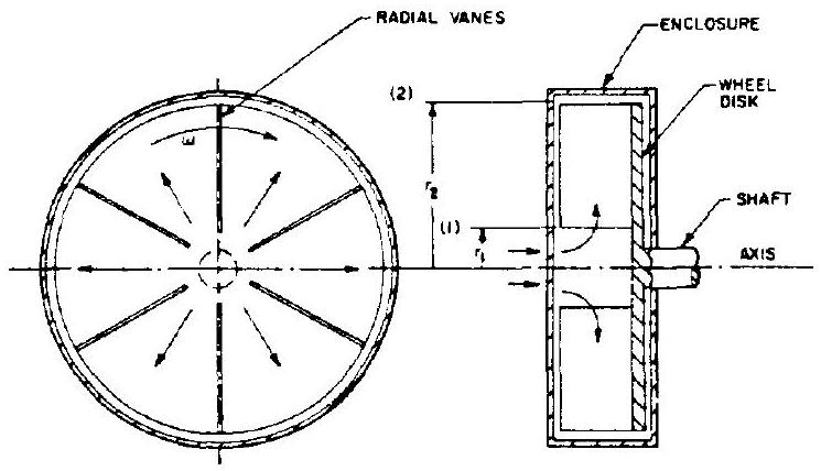 Figure 6-33.-Paddle wheel (schematic).
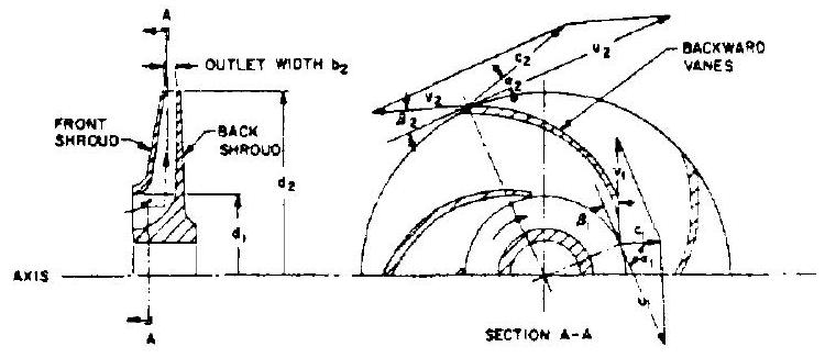 Figure 6-34.-Typical shrouded centrifugal impeller with backward curved vanes.
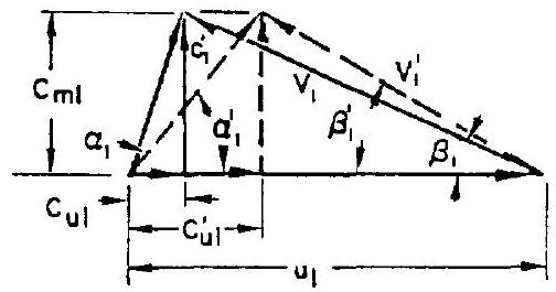 INLET VELOCITY DIAGRAM
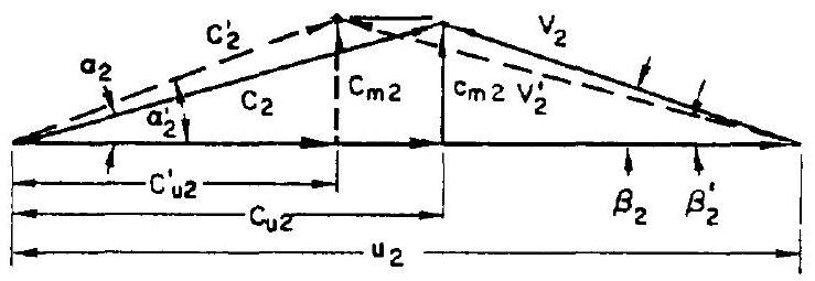 OUTLET VELOCITY DIAGRAMS
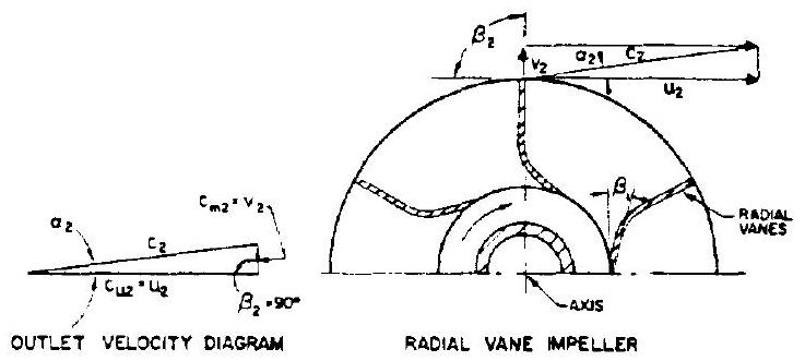 Figure 6-36.-Typical radial vane impeller and its outlet velocity diagram.
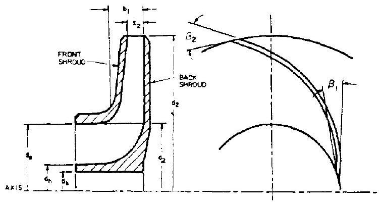 Figure 6-37.-Basic layout of a typical radial- flow impeller with backward curved vanes.
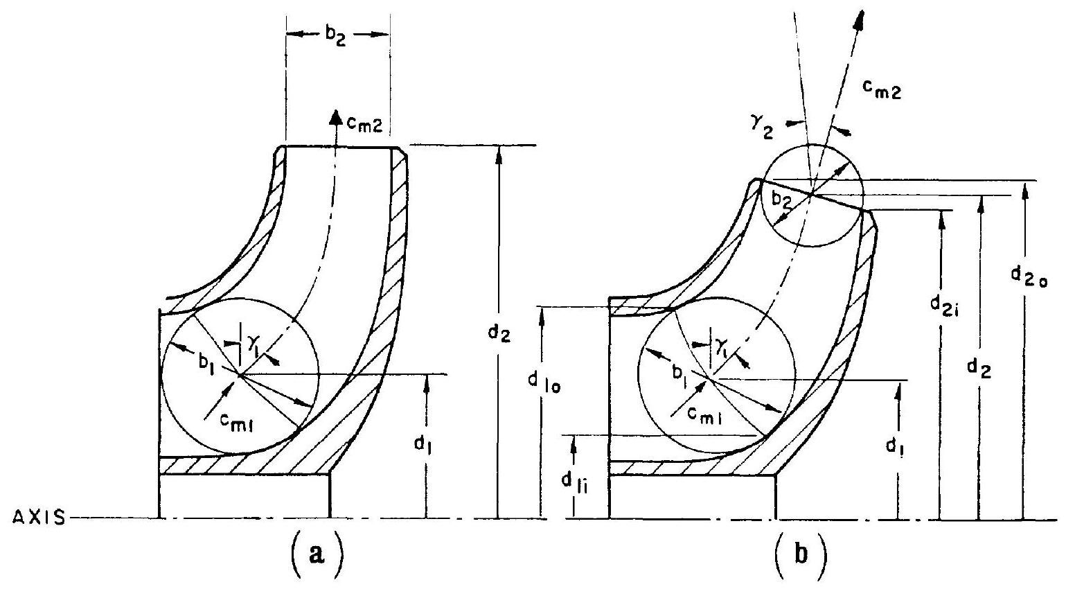 Figure 6-38.-(a) Radial-flow impeller with mixed-flow vanes at the impeller entrance; (b) Mixed-flow impeller.
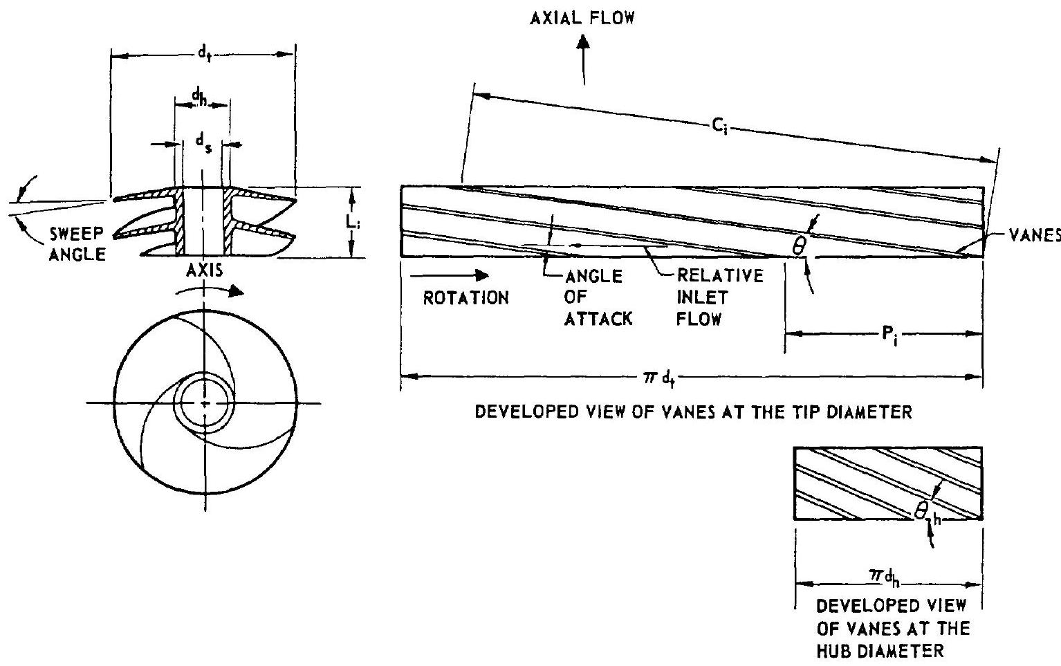 Figure 6-39.-Elements of a typical inducer design (three-vanes; cylindrical hub and tip contour).
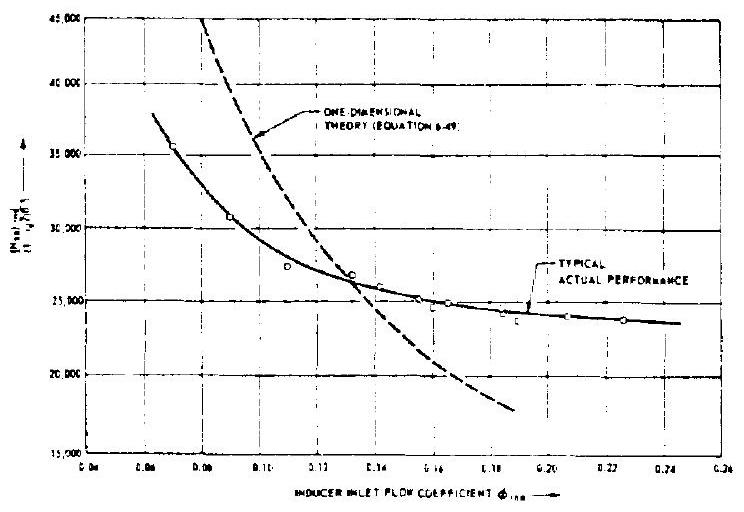 Figure 6-40.-Relation between inducer inlet flow coefficient and inducer suction specific speed.
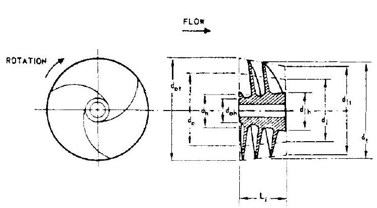 Figure 6-41.-Taper contour inducer.
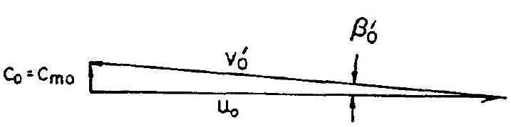 INLET VELOCITY DIAGRAM
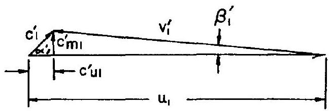 OUTLET VELOCITY DIAGRAM
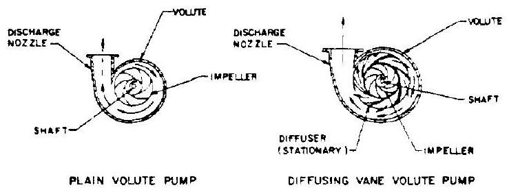 Figure 6-43.-Plain volute and diffusing vane volute centrifugal pump casings.
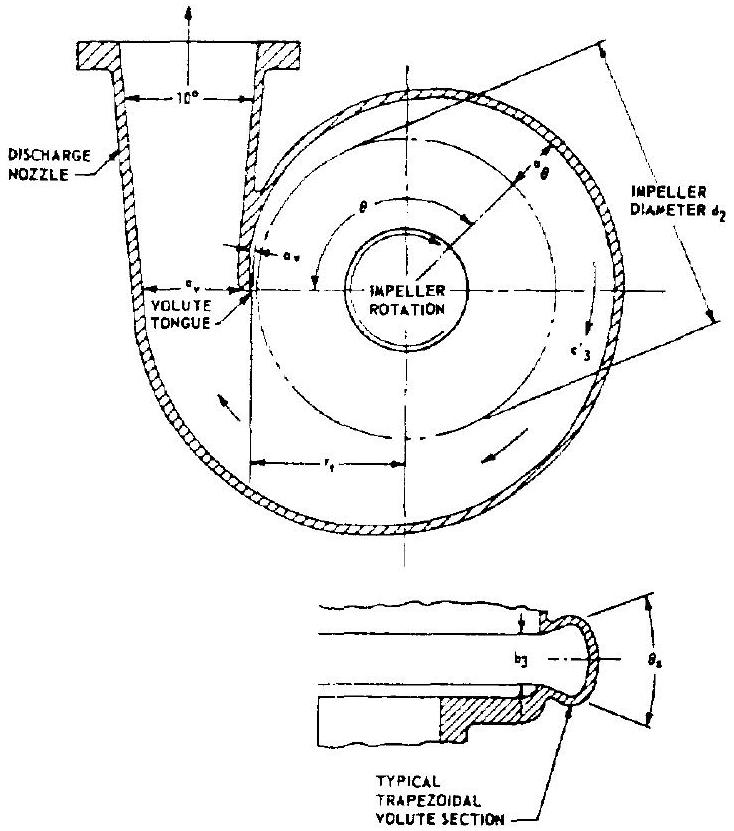 Figure 6-44.-Plain volute casing of a centrifugal pump.
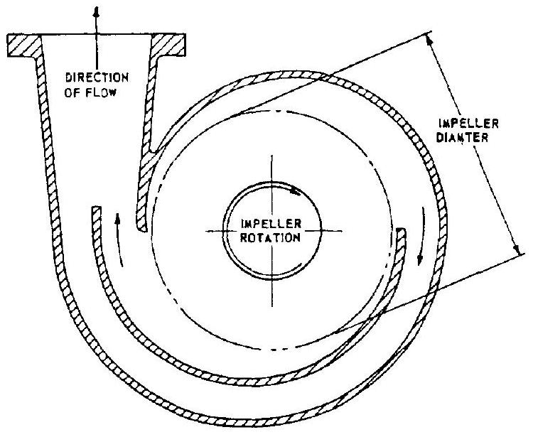 Figure 6-45.-Typical single discharge, opposed double-volute casing of a centrifugal pump.
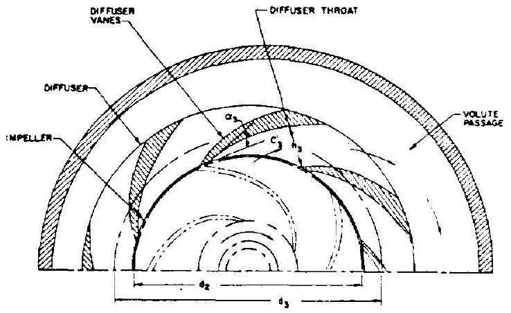 Figure 6-46.-Typical layout of the diffuser for a centrifugal pump volute casing.
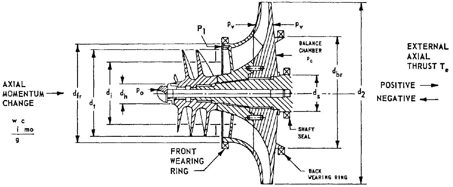 Figure 6-47.-Balancing axial thrusts of a centrifugal pump by the balance chamber method.
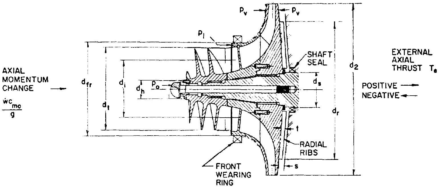 Figure 6-48.-Balancing axial thrusts of a centrifugal pump by the radial rib method.